What Surfacing Is
From a distance, a dense point cloud already looks like a solid surface. But software cannot drape a texture over loose points, slice a section through them, or compute a watertight volume from them. For most work you need an actual surface: a mesh — a web of triangles (or polygons) whose faces form a continuous skin. Surfacing is the step that builds that skin from the points.
Every engine on this page takes the same input — positions, and sometimes color and normals — and produces the same kind of output: surface vertices joined into triangles or general polygons, optionally carrying the cloud’s color. What differs is how they decide which points to connect, and that choice is everything.
Two Questions That Pick the Method
The engines look different, but they mostly sort along two questions about your data and your goal.
1. Is your surface a height field, or a full 3D shape?
Terrain — the ground, a field, a road, a stockpile seen from above — has one height per location. Surfaces like that are “2.5D” height fields, and the simplest, fastest engines exploit that. An object with overhangs, a building facade, a tunnel, a tree, or a statue is fully 3D: a single XY spot can have many surfaces stacked above it, so it needs an engine that works in true 3D.
2. Should the surface pass through the points, or smooth them?
If your data is clean and you trust every point, an interpolating engine that runs the surface exactly through the points keeps all the detail. If the cloud is noisy, or you want a clean watertight result, an approximating engine that fits a surface near the points — averaging out the scatter — gives a far better mesh.
Normals: usually handled for you
A few engines (Poisson, RBF, Hoppe, and greedy projection) need a normal at every point — the direction the surface faces — to tell inside from outside. NDEVR estimates and orients normals automatically when they are missing, so you rarely set them by hand; but the quality of those normals is what makes or breaks those methods.
The Surfacing Engines
Each engine below is one option NDEVR can run on a selection of points. They are grouped from the simplest height-field methods to the full-3D reconstructions.
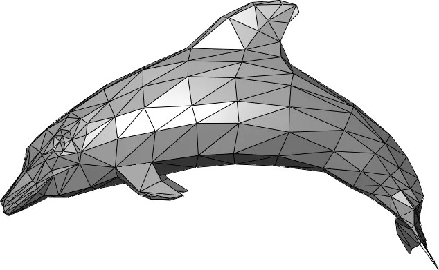
Delaunay triangulation (TIN)
The classic terrain method. The points are projected onto a horizontal plane and connected into the “best” non-overlapping triangles — the Delaunay criterion favors fat, well-shaped triangles over thin slivers — then the triangle network is draped back over the points’ real elevations. The result is a Triangulated Irregular Network (TIN) that passes exactly through every input point. The triangulated mesh at the top of this page is built this way.
- Strengths — very fast; exact (honors every point); deterministic; the natural base for contours, slope/volume analysis, and DTM/DSM terrain models.
- Limitations — strictly 2.5D: it cannot represent overhangs, vertical walls, or the underside of anything. Noise and stray points become spikes, because the surface is forced through them.
- Key setting — essentially parameter-free; you control quality mostly by thinning/cleaning the cloud first and by the boundary you surface within.
- Reach for it when — you have ground or top-surface data and want a fast, faithful terrain model.
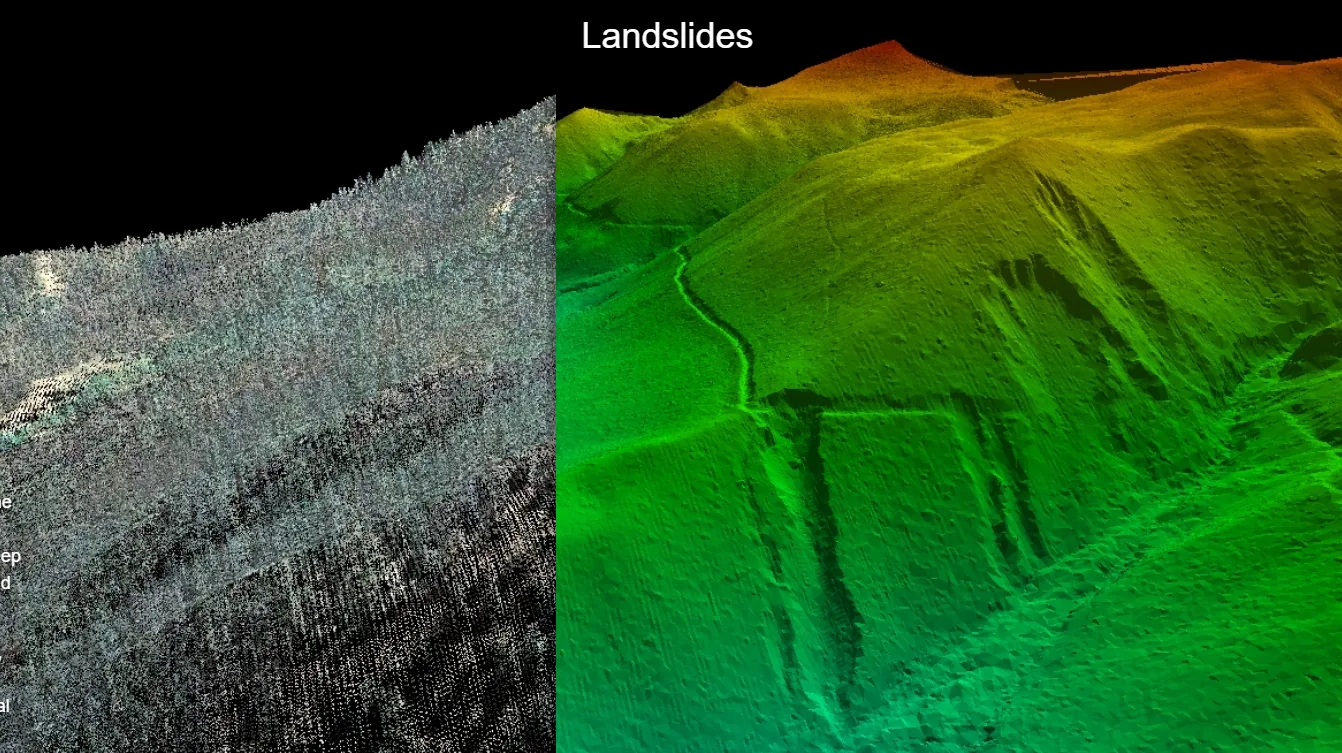
Cloth simulation (CSF)
The Cloth Simulation Filter turns the cloud upside down and drops a virtual sheet of “cloth” onto it under gravity. The cloth settles onto the points, and a stiffness setting keeps it from sagging into every dip — so it traces out the underlying ground while ignoring vegetation, vehicles, and buildings. It is the standard tool for extracting bare earth, and the settled cloth doubles as a smooth ground surface.
- Strengths — excellent, robust ground extraction under trees and clutter; intuitive; few parameters; no normals needed; smooths out noise.
- Limitations — terrain only (a single 2.5D surface); iterative, so slower than a TIN; needs a little tuning on very steep or terraced ground; fine ground detail is smoothed.
- Key setting — cloth resolution (the spacing of the simulated grid): finer resolution follows more terrain detail at higher cost, plus a “steep slopes” option for rugged sites.
- Reach for it when — you need a clean ground model, or to separate ground from everything else, in a vegetated or messy scan.
A two-sided variant runs the cloth from the top and the bottom and joins the two drapes into a single closed shell — a quick way to wrap a stockpile or mound in a closed surface (for volume or visualization) without needing normals. It costs roughly twice as much and can self-intersect in deep concavities, so it is a convenience wrap, not a true 3D reconstruction.
Marching cubes (voxel grid)
NDEVR’s native full-3D method. The points are dropped into a 3D grid of cells (voxels); each cell accumulates how much “stuff” it contains, and the marching cubes algorithm then extracts a surface wherever that density crosses a threshold. Because it works on a volume rather than a plane, it happily wraps overhangs and closed shapes — and it carries the cloud’s color straight through to the mesh.
- Strengths — full 3D; very robust to noise and outliers (they average into the grid); needs no normals; preserves color; predictable.
- Limitations — blocky if the grid is coarse; memory and time climb quickly as you refine it; tends to fill small concavities and holes; the surface floats near the points rather than through them.
- Key setting — grid resolution (voxel size): the master trade-off between detail and memory.
- Reach for it when — you have a noisy, dense, full-3D cloud (often without reliable normals) and want a robust mesh that keeps color.
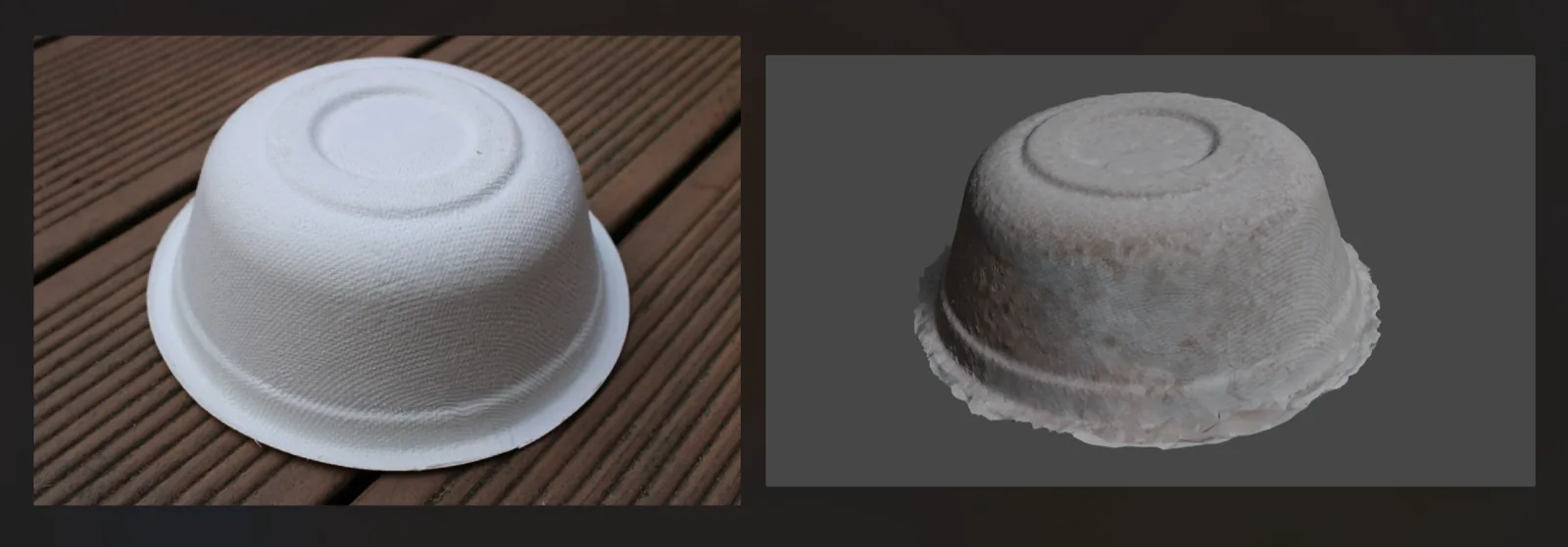
Poisson reconstruction
The go-to for turning a dense scan of a solid object into a clean mesh. Poisson treats the oriented points as samples of the surface’s gradient and solves a single global equation for the smooth surface whose normals best match them. The result is smooth and watertight, and it gracefully bridges gaps and holes. It needs a normal at every point (computed automatically if absent).
- Strengths — smooth, watertight surfaces; outstanding on dense, noisy scans of objects, people, and rooms; fills holes naturally.
- Limitations — needs good normals; because it always closes the surface, it “balloons” out past the data and usually needs trimming; rounds off genuinely sharp edges; slower; the closed-surface assumption is wrong for open terrain.
- Key setting — octree depth: higher depth resolves finer detail (more memory and time, and more sensitivity to noise); lower depth is smoother and coarser.
- Reach for it when — you have a dense cloud of a closed object and want one smooth, watertight mesh.
Implicit grids: RBF & Hoppe
Two more full-3D reconstructions that, like Poisson, build an invisible signed-distance field (positive outside the surface, negative inside) and then run marching cubes on a regular grid to pull out the zero-level surface. They differ in how that field is defined. RBF (radial basis functions) fits one smooth global function through the points — good at extrapolating across gaps. Hoppe sets the distance from the nearest point’s tangent plane — fast and local. Both need oriented normals.
- Strengths — smooth implicit surfaces; RBF bridges sparse gaps well; Hoppe is fast and direct; useful alternatives when Poisson is not the right fit.
- Limitations — need normals; a regular grid uses more memory than Poisson’s octree; Hoppe is sensitive to inconsistent normals (it can leave holes); RBF slows down on very large clouds.
- Key setting — grid resolution (voxel size), plus an iso-level offset to inflate or shrink the surface slightly.
- Reach for it when — you want an implicit reconstruction with specific behavior: RBF to fill gaps in sparse data, Hoppe for a quick signed-distance mesh on clean, well-oriented points.
Greedy projection
A direct, “connect-the-dots” triangulation in 3D. Greedy projection starts from a seed triangle and grows the mesh outward, repeatedly stitching each point to nearby neighbors that satisfy distance and angle limits, until a front of triangles has spread across the cloud. Like Delaunay, it is interpolating — the mesh runs through the actual points, so it keeps fine detail and does not smooth. It needs normals.
- Strengths — fast; keeps the original points (exact, detail-preserving); does not smooth; great on clean, evenly-sampled scans.
- Limitations — needs normals; leaves holes in sparse, uneven, or overlapping regions; struggles with noise; the result is not watertight, and local choices can create stray non-manifold patches.
- Key setting — search radius (the longest edge / neighborhood it will bridge): too small leaves holes, too large stitches across gaps it should not.
- Reach for it when — you have a clean, fairly uniform cloud and want a faithful, detail-preserving mesh fast, with no smoothing.
Choosing the Right One
Answer the two questions from above — height field or full 3D, and through-the-points or smoothed — and this table narrows it to one or two engines. “Through” means the surface passes through every point (interpolating); “near” means it fits a surface close to them (approximating).
| Engine | Shape | Points | Normals | Noise | Watertight | Best for |
|---|---|---|---|---|---|---|
| Delaunay / TIN | 2.5D | Through | No | Poor | No | Terrain, ground & top surfaces, contours, volumes |
| Cloth (CSF) | 2.5D | Near | No | Good | No | Bare-earth from vegetated or cluttered scans |
| Two-sided CSF | 3D (closed) | Near | No | Good | Roughly | A quick closed shell around a pile or mound |
| Marching cubes (grid) | 3D | Near | No | Excellent | Yes | Noisy full-3D clouds; keeps color |
| Poisson | 3D | Near | Auto | Excellent | Yes | Dense scans of solid objects → smooth watertight mesh |
| RBF / Hoppe | 3D | Near | Auto | Good | Mostly | Implicit reconstruction; RBF fills gaps, Hoppe is fast |
| Greedy projection | 3D | Through | Auto | Poor | No | Clean, even clouds; faithful detail, fast |
A quick rule of thumb: for terrain, start with a TIN, or cloth simulation if you must strip vegetation first. For a scanned object, start with Poisson; drop to marching cubes if your normals are unreliable, or to greedy projection if the data is clean and you want to preserve every point.
After Surfacing
A raw mesh is rarely the final product. A few finishing steps apply across every engine:
- Normals — NDEVR estimates and orients per-point normals automatically for the engines that need them; their consistency is what keeps a reconstruction from turning inside-out.
- Color — the cloud’s color can be carried onto the surface, or sampled from the nearby points after the fact, so the mesh keeps its real-world appearance.
- Cleanup — nearby duplicate vertices can be merged, and the surface can be clipped to a boundary you select — useful for trimming the over-extended edges Poisson and the implicit methods tend to produce.
- Simplify — a dense mesh can be decimated down to a lighter one for modeling, sharing, or the web, while keeping its shape.
Pick the engine that matches your data, and the point cloud you captured becomes a surface you can build on — a terrain model, a watertight scan, or a faithful as-built mesh. To go back a step and understand the input, see What is a Point Cloud?; for how clouds are captured in the first place, see What is LiDAR? and What is Photogrammetry?