Waves That Add
Two water waves that meet do not bounce off each other. They pass through each other, and where they overlap the surface height is the sum of the two. Peak on peak gives a taller peak. Peak on trough gives flat water. Sound does the same, which is why a chord sounds like one blended tone, and why noise-cancelling headphones can silence a steady drone by playing a copy of it upside down.
Quantum amplitudes add in the same way, with one difference. A water wave is a height you can measure directly. A quantum amplitude cannot be measured on its own. What you measure are outcomes, and the square of the amplitude gives their probability. The sign of the amplitude shows up only when two paths to the same outcome combine.
A Particle That Interferes With Itself
In 1989 a team at Hitachi led by Akira Tonomura sent electrons one at a time through an electron biprism, the electron-microscope equivalent of a pair of slits, and recorded where each one landed. Each electron arrived as a single dot. There was never a smear or half an electron. But as the dots accumulated, bands appeared: regions the electrons favoured and regions they avoided. Only one electron was in the apparatus at a time, so nothing was interfering with each electron except itself. A Bologna group had shown the same build-up with coarser equipment in 1974.
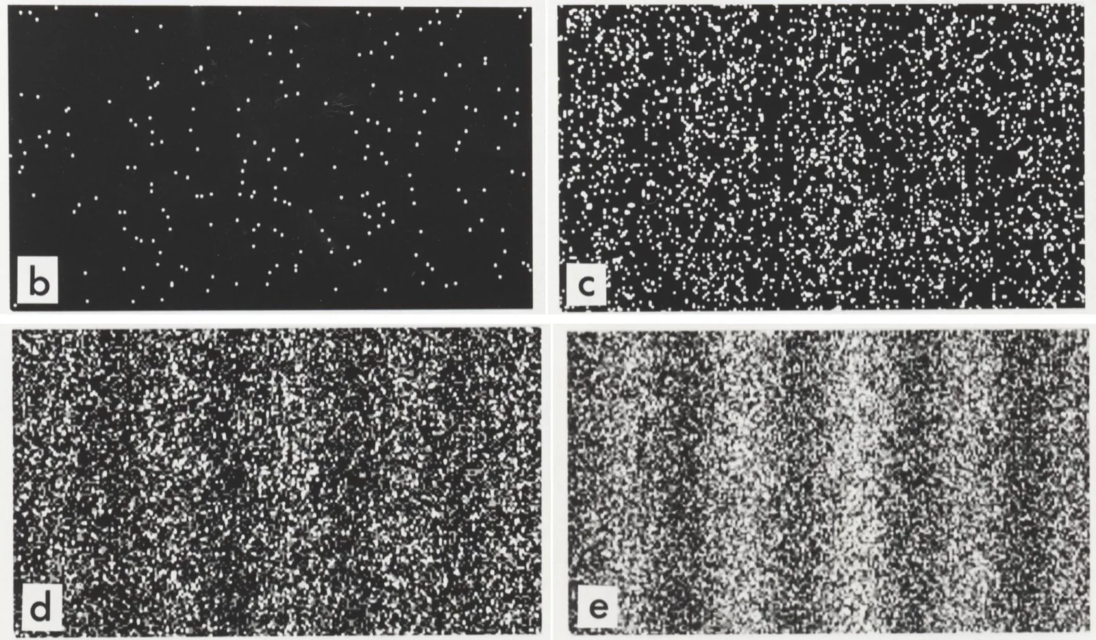

The explanation is the one from the previous section. Each electron has an amplitude for every path to every point on the screen. Where the amplitudes for the two paths arrive with the same sign they reinforce, and electrons are likely to land. Where they arrive with opposite signs they cancel, and electrons never land. Each individual electron still lands in one place, chosen at random with those odds. Block one path and the bands vanish, because there is no longer a second amplitude to cancel the first.
Measurement Creates the Result
An ordinary measurement reveals something that was already true. A brick has a weight whether or not it sits on a scale. A quantum measurement is different. Before the measurement the electron had amplitudes for many positions; it did not have one position that the detector then found. The detector produced one. Repeat the experiment with identically prepared electrons and the results differ, and no extra information about the preparation would let you predict which result you will get.
A coin toss looks similar but is not. A coin’s result is fixed by its launch and the air; the randomness is our ignorance. Quantum randomness is not ignorance of a hidden value. Experiments on entangled particles, described in What is Quantum Entanglement?, rule out the idea that the value was there all along, at least for any hidden value that stays local.
After a measurement the state is the outcome that was found. Measure the same qubit again and you get the same answer. This is usually called collapse. It is why quantum programs measure at the end rather than during the computation: every measurement throws away the amplitudes that interference needed.
The uncertainty principle is a different fact
Heisenberg’s principle limits how precisely two complementary properties, such as position and momentum, can be known at the same time. It is not the reason a single measurement is random; superposition is. The related fact that matters for security is that a qubit cannot be measured in two incompatible ways at once. Quantum key distribution relies on that, and it is a separate technology from the post-quantum encryption OWL uses, which is ordinary software.
Interference Is the Computation
A quantum computer is a device for steering interference. Its gates move amplitudes around so that, for the answer you want, the contributions arriving from different paths share a sign and add, while for every other answer they arrive with mixed signs and cancel. The simplest example uses one qubit and two Hadamard gates, the gate that splits an amplitude into two equal branches. Run H twice and the second H splits each branch again, so each readout receives two contributions.
| Circuit | Readout | From the |0⟩ branch | From the |1⟩ branch | Total | Probability |
|---|---|---|---|---|---|
| H, then H | 0 | +0.5 | +0.5 | 1 | 100% |
| 1 | +0.5 | −0.5 | 0 | 0% | |
| H, then Z, then H | 0 | +0.5 | −0.5 | 0 | 0% |
| 1 | +0.5 | +0.5 | 1 | 100% |
Two random-looking steps combine into a certain answer, and one hidden sign flip between them selects the other answer. Every quantum algorithm is a larger version of this table. Shor’s algorithm uses a Fourier transform over thousands of qubits so that contributions from a repeating pattern add up only at the period; Shor, Grover and the Quantum Speedup walks through it. The animated walkthrough on What is a Quantum Computer? shows these two passes in motion as step 5.
Sources & Further Reading
- A. Tonomura, J. Endo, T. Matsuda, T. Kawasaki and H. Ezawa, “Demonstration of single-electron buildup of an interference pattern”, American Journal of Physics 57, 117 (1989). The earlier Bologna experiment: P. G. Merli, G. F. Missiroli and G. Pozzi, American Journal of Physics 44, 306 (1976).
- R. P. Feynman, The Feynman Lectures on Physics, Volume III, Chapter 1: Quantum Behavior: the double-slit experiment as the one essential mystery.
- The Quantum Atlas: Superposition, Measurement and The Uncertainty Principle, Joint Quantum Institute, University of Maryland.
- M. A. Nielsen and I. L. Chuang, Quantum Computation and Quantum Information (Cambridge University Press, 2010), sections 1.2 and 2.2: the measurement postulate and the amplitude rules.